
Plate artifacts and corrections#
Plates drift, well position matters, and cell count affects most features. This page looks for those artifacts
on a real screen, pki: eight plates of kinase inhibitors from the JUMP pilot [Chandrasekaran et al., 2023]. It
removes them and measures whether removing them helped.
Every correction here can make results worse on a given dataset. The last section shows a real case where sphering, a standard step of the pipeline, cuts mechanism retrieval by more than three quarters.
import warnings

import numpy as np
import pandas as pd
import scanpy as sc

import mantispy as mt
from mantispy._core.plate import well_col, well_row

wells = mt.ds.pki()
mt.pp.normalize(wells, method="mad_robustize", by="Metadata_Plate", reference="negcon")
mt.pp.feature_select(wells, na_cutoff=0.0)
wells = mt.pp.subset_features(wells)
wells
AnnData object with n_obs × n_vars = 3072 × 850
    obs: 'Metadata_plate_map_name', 'Metadata_broad_sample', 'Metadata_mg_per_ml', 'Metadata_mmoles_per_liter', 'Metadata_solvent', 'Metadata_Plate', 'Metadata_Well', 'Metadata_Site_Count', 'Metadata_Count_Cells', 'Metadata_Count_CellsIncludingEdges', 'Metadata_Count_Cytoplasm', 'Metadata_Count_Nuclei', 'Metadata_Count_NucleiIncludingEdges', 'Metadata_Object_Count', 'Metadata_Barcode', 'Metadata_Supplier', 'Metadata_Supplier_Catalog', 'Metadata_pert_type', 'Metadata_control_type', 'Metadata_CellCount', 'Metadata_SiteCount', 'Metadata_Control', 'Metadata_Compound', 'Metadata_Concentration', 'Metadata_MOA', 'Metadata_Perturbation'
    var: 'object', 'feature_group', 'feature', 'channel', 'scale', 'angle', 'gray_levels', 'radial_bin', 'params', 'is_feature', 'degenerate_scale', 'selected'
    uns: 'mantispy'
    layers: None (.X)
import plotly.io as pio

pio.renderers.default = "notebook_connected"
Position effects#
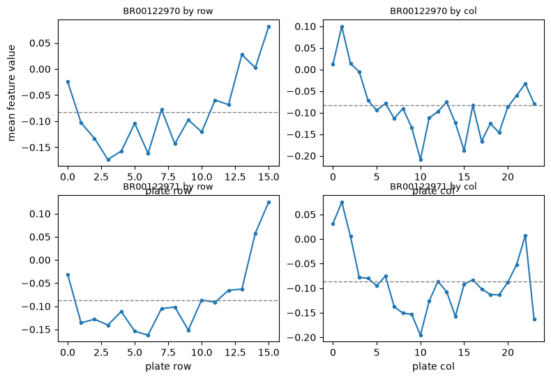
Edge wells evaporate, corners sit at a different temperature, and dispensing drifts along a row.
pl.plate_effects shows the row and column medians of each plate. A position artifact appears as a trend across
rows or columns, while noise scatters around the plate median. Two of the eight plates:
two = wells[wells.obs["Metadata_Plate"].isin(wells.obs["Metadata_Plate"].cat.categories[:2]).to_numpy()].copy()
mt.pl.plate_effects(two);
correct_plate_position fits Tukey’s median polish to the row and column effects of each plate and subtracts
them. Median polish is used instead of a mean-based fit so that a few extreme wells do not define the gradient.
How much position explains, before and after, as each feature’s correlation with the row and the column it sits
in:
rows = np.array([well_row(well) for well in wells.obs["Metadata_Well"]])
columns = np.array([well_col(well) for well in wells.obs["Metadata_Well"]])


def position(adata):
    """Median and largest absolute correlation of a feature with its well's row and column."""
    values = np.asarray(adata.X, dtype=float)
    result = {}
    for name, axis in (("row", rows), ("column", columns)):
        r = np.abs([np.corrcoef(axis, values[:, j])[0, 1] for j in range(values.shape[1])])
        result[f"{name}: median |r|"] = round(float(np.nanmedian(r)), 3)
        result[f"{name}: largest |r|"] = round(float(np.nanmax(r)), 3)
    return result


corrected = mt.pp.correct_plate_position(wells, copy=True)
pd.DataFrame({"before": position(wells), "after": position(corrected)})
| before | after | |
|---|---|---|
| row: median |r| | 0.055 | 0.012 |
| row: largest |r| | 0.316 | 0.132 |
| column: median |r| | 0.070 | 0.021 |
| column: largest |r| | 0.692 | 0.131 |
Position explains little of most features and a lot of a few. Before correction the median feature correlates with its well’s column at 0.07, and the most affected one at 0.69; median polish takes the largest correlation with the row or the column to about 0.13.
If treatments are laid out by column, fit the effects on the controls only, with
reference="negcon", so that treatment effects are not absorbed into a column effect and
subtracted.
This has a limit. A median polish can only fit a column effect for columns that contain reference rows, and most layouts put the controls in a few fixed columns, such as 1 and 2 or 23 and 24. With controls in four of twenty-four columns there is no control-only column effect to fit. Row effects still work, because controls in an edge column span every row. For column effects on a column-wise layout, the design has confounded the effect you want to correct, and the fix is a randomized layout on the next plate.
Confounders#
Cell count is the most common one: a sparse well looks different from a confluent one regardless of treatment.
regress_out fits each feature against the confounder within each plate and keeps the residual.
The fit has to be made on wells whose density varies for technical reasons only. In a compound screen the
treatments change density too, and a compound that thins its wells usually has a phenotype of its own, so a fit
over every well mistakes that phenotype for a density effect. reference="negcon" fits on the DMSO wells, keeps
them where normalization centred them, and corrects a well sparser or denser than any control as if it sat at the
edge of their range rather than by extrapolating.
counts = wells.obs["Metadata_CellCount"].to_numpy(dtype=float)
plates = wells.obs["Metadata_Plate"].astype(str).to_numpy()
control = wells.obs["Metadata_Control"].to_numpy(dtype=bool)


def density(adata):
    """How much of each feature follows the cell count, and whether the controls stay centred."""
    values = np.asarray(adata.X, dtype=float)
    within = []
    for plate in np.unique(plates):
        rows = (plates == plate) & control
        r = [np.corrcoef(counts[rows], values[rows, j])[0, 1] for j in range(values.shape[1])]
        within.append(np.nanmedian(np.abs(r)))
    every = [np.corrcoef(counts, values[:, j])[0, 1] for j in range(values.shape[1])]
    return {
        "DMSO wells, within plates: median |r|": round(float(np.median(within)), 3),
        "every well: median |r|": round(float(np.nanmedian(np.abs(every))), 3),
        "DMSO wells off centre": round(float(np.median(np.abs(np.median(values[control], axis=0)))), 3),
    }


print(
    "median cells per well, by plate:",
    wells.obs.groupby("Metadata_Plate", observed=True)["Metadata_CellCount"].median().to_dict(),
)

fit_on_everything = mt.pp.regress_out(wells, keys=("Metadata_CellCount",), by="Metadata_Plate", copy=True)
fit_on_controls = mt.pp.regress_out(
    wells, keys=("Metadata_CellCount",), by="Metadata_Plate", reference="negcon", copy=True
)
pd.DataFrame(
    {
        "before": density(wells),
        "fit on every well": density(fit_on_everything),
        "fit on the DMSO wells": density(fit_on_controls),
    }
)
median cells per well, by plate: {'BR00122970': 1974.5, 'BR00122971': 1956.0, 'BR00122972': 607.5, 'BR00122973': 602.5, 'BR00122974': 1640.0, 'BR00122975': 1631.0, 'BR00122977': 1820.0, 'BR00122978': 1803.5}
| before | fit on every well | fit on the DMSO wells | |
|---|---|---|---|
| DMSO wells, within plates: median |r| | 0.179 | 0.193 | 0.000 |
| every well: median |r| | 0.142 | 0.546 | 0.132 |
| DMSO wells off centre | 0.000 | 0.409 | 0.014 |
Two of the eight plates hold about a third of the others’ cells. Fitted on every well, each plate’s fit is
re-expressed at the density of the whole screen, which those two plates never reach, so their correction is an
extrapolation, and regress_out warns about it. The result follows the cell count more closely than before across
the screen, 0.55 against 0.14, and the DMSO wells end 0.41 off the centre normalization gave them.
Fitted on the DMSO wells, the correction removes the count’s pull on them, zero by construction since the fit was made on them, and leaves them centred. Across every well the correlation stays about where it was. What remains there is mostly the treatments’ own effect: a compound that thins its wells also changes the cells that are left, and a correction for technical density should not remove that.
Missing values stay missing. Imputing them for the regression and writing the fitted value back would make an unmeasured value look like a real measurement.
Plates as batches#
A batch effect moves the controls too. pl.control_drift projects the control wells onto components fitted on the
controls alone, so if the controls of different plates land in different places, the reference itself shifts
between them.
mt.pl.control_drift(wells, groupby="Metadata_Plate");
Measuring the result#
mt.metrics scores a representation with several metrics. Batch-mixing metrics and biological-signal metrics
trade off against each other, and a correction that improves one at the expense of the other has not helped.
Normalizing each plate against its own controls is itself a batch correction. Here it is measured against one normalization pooled over the whole screen, on the same features:
pooled = mt.ds.pki()
mt.pp.normalize(pooled, method="mad_robustize", by=None, reference="negcon")
pooled = pooled[:, wells.var_names].copy()

sc.pp.pca(wells, n_comps=20)
sc.pp.pca(pooled, n_comps=20)
wells.obsm["X_pooled"] = pooled.obsm["X_pca"]

table = mt.metrics.evaluate_correction(
    wells, reps=("X_pooled", "X_pca"), label_key="Metadata_Perturbation", batch_key="Metadata_Plate"
)
table
| metric | representation | key | value | better | |
|---|---|---|---|---|---|
| 0 | silhouette_label | X_pooled | Metadata_Perturbation | 0.468931 | higher |
| 1 | silhouette_batch | X_pooled | Metadata_Plate | 0.871798 | higher |
| 2 | ilisi | X_pooled | Metadata_Plate | 1.810165 | higher |
| 3 | clisi | X_pooled | Metadata_Perturbation | 4.944914 | lower |
| 4 | pc_regression | X_pooled | Metadata_Plate | 0.818234 | lower |
| 5 | silhouette_label | X_pca | Metadata_Perturbation | 0.373248 | higher |
| 6 | silhouette_batch | X_pca | Metadata_Plate | 0.833440 | higher |
| 7 | ilisi | X_pca | Metadata_Plate | 2.572630 | higher |
| 8 | clisi | X_pca | Metadata_Perturbation | 4.465037 | lower |
| 9 | pc_regression | X_pca | Metadata_Plate | 0.025963 | lower |
mt.pl.metrics(table);
Check the better column: two of the five metrics are better when lower. Per-plate normalization takes the plate’s
share of the variance from 82% to 3%, and a well’s neighbours come from more plates, an iLISI of 2.6 against 1.8.
The label and batch silhouettes go the other way, 0.37 against 0.47 and 0.83 against 0.87. The metrics trade off, which is why the pages that
follow judge a correction by retrieval, the question a screen asks.
pl.batch_variance shows the plate’s share per component, which tells you where in the embedding it sits.
mt.pl.batch_variance(wells, keys=["Metadata_Plate", "Metadata_Perturbation"], use_rep="X_pca");
Harmony, the last step of the JUMP recipe, corrects an embedding rather than the features.
Reproducing across laboratories runs it on JUMP and measures the result.
For a correction on the features instead of an embedding, sc.pp.combat is the usual choice.
Sphering, and a correction that makes things worse#
Sphering is typical variation normalization. The covariance of the negative controls describes variation that is
not of interest, and whitening removes it, leaving the variation caused by the perturbations. ZCA-cor is the
default because it rotates back into the original feature basis, so the columns still match var.
Sphering needs more control wells than features. BBBC021 [Ljosa et al., 2013] has few control wells for the features that survive selection, so its control covariance is singular. Score mechanism retrieval with and without sphering, with the not-same-compound rule from Mechanism of action.
def not_same_compound(adata):
    """Not-same-compound mechanism retrieval on one signature per treatment."""
    treated = adata[~adata.obs["Metadata_Control"].to_numpy()].copy()
    signatures = mt.tl.consensus(treated, method="median", min_replicates=1)
    signatures = signatures[signatures.obs["Metadata_MOA"].notna().to_numpy()].copy()
    mt.tl.nn_moa_classify(signatures, scheme="nsc")
    return round(signatures.uns["mantispy"]["moa"]["accuracy"], 3)


bbbc = mt.ds.bbbc021()
mt.pp.normalize(bbbc, method="mad_robustize", by="Metadata_Plate", reference="negcon")
mt.pp.feature_select(bbbc, na_cutoff=0.0)
bbbc = mt.pp.subset_features(bbbc)

sphered = bbbc.copy()
with warnings.catch_warnings(record=True) as caught:
    warnings.simplefilter("always")
    mt.pp.sphere(sphered, method="ZCA-cor", reference="negcon")
print(caught[0].message)

{
    "control wells": int(bbbc.obs["Metadata_Control"].sum()),
    "features": bbbc.n_vars,
    "without sphering": not_same_compound(bbbc),
    "with sphering": not_same_compound(sphered),
}
sphering is fitted on 330 reference rows for 343 features. With fewer rows than features the covariance is singular and the transform amplifies noise. Select fewer features first, or use more controls.
{'control wells': 330,
 'features': 343,
 'without sphering': 0.777,
 'with sphering': 0.175}
Sphering cuts not-same-compound accuracy from 0.78 to 0.18, a loss of more than three quarters, on 330 control wells for 343 features. mantispy’s sphering is tested against pycytominer’s, so pycytominer should show the same drop.
Measure a correction on the question the screen asks before adopting it. For this dataset, either select fewer features so the control covariance is well determined, or skip sphering.
Next: Is the screen any good?