JUMP-Lite

jump_lite() reads JUMP-Lite Target-2 [Muñoz et al., 2026]: four plates of the JUMP Target-2 plate map, one from each of four laboratories, with the same 1,536 wells measured six ways. Four are learned embeddings, one is the same architecture as one of them with untrained weights, and cp_measure is a CellProfiler-equivalent feature set. jump_lite_targets() returns the RefChemDB gene annotations of its compounds, in the shape known_relationships() reads.

Source

Three things about how the features were made bound every result computed from them.

• The images are lossy. Every one of the six blocks was computed on JPEG-XL medium-quality images. Texture measurements and convolutional features are the two things most sensitive to compression, so this is not a neutral choice, and it is a property of the benchmark rather than of your screen.

• One field of view per well. Full Target-2 acquires nine; JUMP-Lite keeps one. So every cell count below is cells in one field, and Bringing your own embedding says how to aggregate a model’s per-field output when there is more than one.

• Only one of the six blocks needed segmentation. cp_measure measures objects, so it needs a nucleus and a cell body found for every cell. The five embeddings read the whole field and segment nothing. That is the real difference between the embeddings and cp_measure, and it cuts both ways.

Used in

• Bringing your own embedding

• Which measurements moved

• Learned embeddings against CellProfiler

import mantispy as mt

mt.ds.JUMP_LITE_MODELS

('openphenom', 'dinov2', 'dinov2_random', 'subcell', 'morphem', 'cp_measure')

adata = mt.ds.jump_lite("openphenom")
adata

AnnData object with n_obs × n_vars = 1536 × 384
    obs: 'Metadata_id', 'Metadata_Source', 'Metadata_Batch', 'Metadata_Plate', 'Metadata_Well', 'Metadata_Site', 'Metadata_model', 'Metadata_dataset', 'Metadata_compression', 'Metadata_CellCount', 'Metadata_JCP2022', 'Metadata_InChIKey', 'Metadata_Perturbation', 'Metadata_Perturbation_Type', 'Metadata_Control'
    var: 'object', 'feature_group', 'feature', 'channel', 'scale', 'angle', 'gray_levels', 'radial_bin', 'params', 'is_feature'
    uns: 'mantispy'
    layers: None (.X)

The four batches are four different laboratories running one plate map, which makes this a batch-correction problem with a clean design: whatever separates source_3 from source_6 is not biology, because they received the same compounds in the same wells.

counts = adata.obs.groupby("Metadata_Source", observed=True).agg(
    plate=("Metadata_Plate", "first"),
    wells=("Metadata_Well", "size"),
    controls=("Metadata_Control", "sum"),
    median_cells=("Metadata_CellCount", "median"),
)
# The controls received no compound, so their counts are the site's own density, before any treatment effect.
counts["median_cells, controls"] = (
    adata.obs[adata.obs["Metadata_Control"]].groupby("Metadata_Source", observed=True)["Metadata_CellCount"].median()
)
counts["compounds"] = adata.obs.groupby("Metadata_Source", observed=True)["Metadata_Perturbation"].nunique()
thin = adata.obs["Metadata_CellCount"] < 50
counts["wells under 50 cells"] = thin.groupby(adata.obs["Metadata_Source"], observed=True).sum()
counts

	plate	wells	controls	median_cells	median_cells, controls	compounds	wells under 50 cells
Metadata_Source
source_3	JCPQC016	384	64	264.0	282.0	302	28
source_4	BR00121438	384	64	189.0	210.0	302	61
source_5	ACPJUM012	384	64	336.0	357.0	302	13
source_6	110000293081	384	64	254.0	266.0	302	37

What it looks like

One number per laboratory hides where the wells are. Four 384-well plates, coloured by how many cells were found in the field.

mt.pl.plate(adata, color="Metadata_CellCount", groupby="Metadata_Source", ncols=4)

mt.pl.cell_counts(adata, groupby="Metadata_Source")

row, column = adata.obs["Metadata_Well"].str[0], adata.obs["Metadata_Well"].str[1:].astype(int)
edge = row.isin(["A", "P"]) | column.isin([1, 24])
{
    "share of the plate on the edge": f"{edge.mean():.0%}",
    "share of thin wells on the edge": f"{edge[thin].mean():.0%}",
}

{'share of the plate on the edge': '20%',
 'share of thin wells on the edge': '10%'}

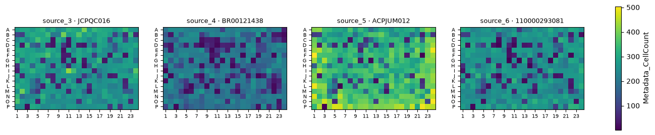
Two facts to know before using it. The sites run at different densities before any compound acts: the control wells, which received none, hold a median of 210 cells at source_4 against 357 at source_5. And the thin wells are not banked against the edge, where evaporation would put them. The edge is a fifth of the plate but holds only a tenth of the thin wells.