The images behind one well

jump_plate() returns two fields of view of well O09 of BR00121438 [Chandrasekaran et al., 2023] as a SpatialData object: the eight channel images of each field, the CellProfiler outlines they were segmented with, and the plate’s cells table. The cells measured from these fields are in jump_cells(), and the well-level profiles of the same plate in jump_target2(). It needs the spatial extra.

Use it if you work from raw Cell Painting images and segmentations rather than tables. Images and segmentations and Quality control use it.

import matplotlib.pyplot as plt
import numpy as np

import mantispy as mt

import warnings

with warnings.catch_warnings():
    warnings.simplefilter("ignore")
    sdata = mt.ds.jump_plate()
sdata

SpatialData object
├── Images
│     ├── 'BR00121438_O09_s1_image': DataTree[cyx] (8, 1080, 1080), (8, 540, 540), (8, 270, 270)
│     └── 'BR00121438_O09_s2_image': DataTree[cyx] (8, 1080, 1080), (8, 540, 540), (8, 270, 270)
├── Labels
│     ├── 'BR00121438_O09_s1_cells': DataArray[yx] (1080, 1080)
│     ├── 'BR00121438_O09_s1_cytoplasm': DataArray[yx] (1080, 1080)
│     ├── 'BR00121438_O09_s1_nuclei': DataArray[yx] (1080, 1080)
│     ├── 'BR00121438_O09_s2_cells': DataArray[yx] (1080, 1080)
│     ├── 'BR00121438_O09_s2_cytoplasm': DataArray[yx] (1080, 1080)
│     └── 'BR00121438_O09_s2_nuclei': DataArray[yx] (1080, 1080)
└── Tables
      └── 'cells': AnnData (284, 1989)
with coordinate systems:
    ▸ 'BR00121438', with elements:
        BR00121438_O09_s1_image (Images), BR00121438_O09_s2_image (Images), BR00121438_O09_s1_cells (Labels), BR00121438_O09_s1_cytoplasm (Labels), BR00121438_O09_s1_nuclei (Labels), BR00121438_O09_s2_cells (Labels), BR00121438_O09_s2_cytoplasm (Labels), BR00121438_O09_s2_nuclei (Labels)
    ▸ 'BR00121438_O09', with elements:
        BR00121438_O09_s1_image (Images), BR00121438_O09_s2_image (Images), BR00121438_O09_s1_cells (Labels), BR00121438_O09_s1_cytoplasm (Labels), BR00121438_O09_s1_nuclei (Labels), BR00121438_O09_s2_cells (Labels), BR00121438_O09_s2_cytoplasm (Labels), BR00121438_O09_s2_nuclei (Labels)
    ▸ 'BR00121438_O09_s1', with elements:
        BR00121438_O09_s1_image (Images), BR00121438_O09_s1_cells (Labels), BR00121438_O09_s1_cytoplasm (Labels), BR00121438_O09_s1_nuclei (Labels)
    ▸ 'BR00121438_O09_s2', with elements:
        BR00121438_O09_s2_image (Images), BR00121438_O09_s2_cells (Labels), BR00121438_O09_s2_cytoplasm (Labels), BR00121438_O09_s2_nuclei (Labels)

The five fluorescence channels

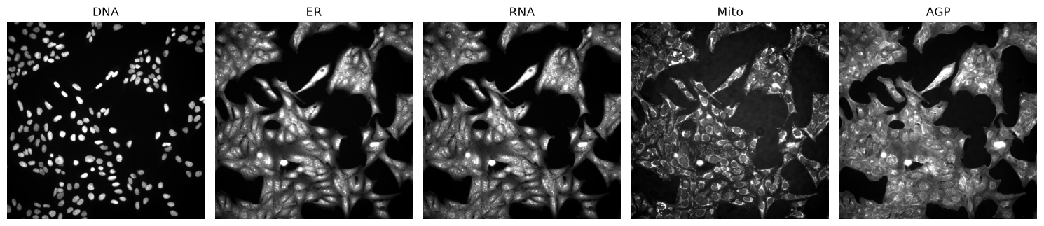
The eight acquisition channels include three brightfield planes; the five Cell Painting fluorescence channels are DNA, the endoplasmic reticulum (ER), RNA, the mitochondria (Mito) and the actin, Golgi and plasma membrane stain (AGP). Each is clipped to its 1st and 99th percentiles for display.

image = sdata.images["BR00121438_O09_s1_image"]["scale0"]["image"]
channels = ["DNA", "ER", "RNA", "Mito", "AGP"]
fig, axes = plt.subplots(1, len(channels), figsize=(15, 3.2))
for ax, channel in zip(axes, channels, strict=True):
    plane = np.asarray(image.sel(c=channel).data)
    low, high = np.percentile(plane, [1, 99])
    ax.imshow(plane, cmap="gray", vmin=low, vmax=high)
    ax.set_title(channel)
    ax.axis("off")
fig.tight_layout()