Learned embeddings against CellProfiler

JUMP-Lite [Muñoz et al., 2026] measured the same 1,536 wells six ways: four learned embeddings, the same architecture as one of them with untrained weights, and cp_measure, a CellProfiler-equivalent feature set. Swapping the feature block is a controlled experiment rather than a change of dataset. The images are lossy and there is one field of view per well, and the dataset page says what that bounds. Bringing your own embedding covers loading one and what var no longer tells you.

import matplotlib.pyplot as plt
import numpy as np
import pandas as pd
import scanpy as sc

import mantispy as mt

classical = mt.ds.jump_lite("cp_measure")
mt.pp.normalize(classical, method="mad_robustize", by="Metadata_Plate", reference="negcon")

import plotly.io as pio

pio.renderers.default = "notebook_connected"

Preparing each block

The embeddings are normalized per plate and not selected, for the reason on Bringing your own embedding. cp_measure is a list of measurements, with the usual pathologies: features that never vary, that duplicate each other, or that run away to enormous values. Holding the selection identical across blocks would be the unfair comparison, not the fair one. Here is what each selection step is worth on it.

PYCYTOMINER = ("variance_threshold", "correlation_threshold", "drop_na_columns", "blocklist")
# feature_select's own default: drop_degenerate, which removes only what normalize flagged, then pycytominer's.
DEFAULT = ("drop_degenerate", *PYCYTOMINER)

selection = {}
for label, operations in {
    "none": ("drop_degenerate", "drop_na_columns"),
    "pycytominer default": DEFAULT,
    "default + drop_outliers": (*DEFAULT, "drop_outliers"),
    "+ noise_removal": (*DEFAULT, "drop_outliers", "noise_removal"),
}.items():
    trial = classical.copy()
    mt.pp.feature_select(trial, operations=operations, na_cutoff=0.0)
    trial = mt.pp.subset_features(trial)
    selection[label] = {
        "features": trial.n_vars,
        "largest |value|": float(np.abs(np.asarray(trial.X)).max()) if trial.n_vars else np.nan,
    }
pd.DataFrame(selection).T

	features	largest |value|
none	1949.0	178622.234375
pycytominer default	540.0	178622.234375
default + drop_outliers	526.0	456.745605
+ noise_removal	0.0	NaN

Left alone, cp_measure carries values of order 1e5, which survive a robust per-plate normalization because they are not constant, merely enormous. The pycytominer default cuts the block to about a quarter of its features and leaves the largest value where it was. drop_outliers, which is in pp.OPERATIONS and not in the default set, removes only fourteen more features and brings the largest value down about four-hundred-fold. noise_removal empties the block: its cutoff is an absolute standard deviation, and on the scale mad_robustize leaves no feature falls under it.

So cp_measure gets the standard selection plus drop_outliers, and the embeddings get none.

Comparing six feature sets

The question is not whether an embedding works, but how it compares with the alternatives on the same wells. Two readouts:

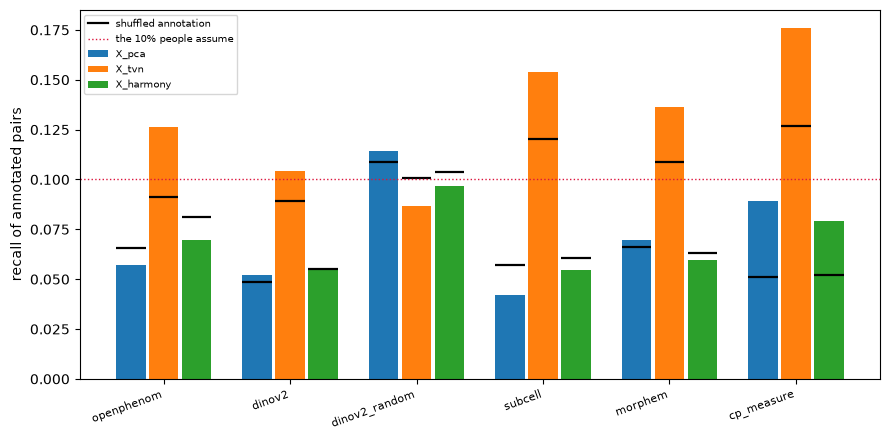
• tl.map — mean average precision. Rank every other profile by similarity to a query and ask whether its replicates come first. The pairs are defined so that a replicate must come from a different laboratory, which is the cross-site reproducibility question, and copairs gives every compound a permutation p-value that is then BH-corrected. This is the metric the JUMP benchmarks report [Arevalo et al., 2024, Kalinin et al., 2025], and it is the only one of the two that scales: the similarity-matrix readouts build a dense n-by-n matrix.

• metrics.known_relationships — of the compounds annotated to act on the same gene, how many end up in either tail of the similarity distribution?

Each is measured under three alignments: the principal components alone, pp.tvn, and pp.harmony, which ranked top-three in every scenario of the batch-correction benchmark [Arevalo et al., 2024] and is the last step of the JUMP recipe. pp.harmony needs the optional extra, pip install 'mantispy[harmony]'.

targets = mt.ds.jump_lite_targets()


def align(wells):
    """The three alignments every block is compared under: none, TVN and Harmony, on the same 50 components."""
    sc.pp.pca(wells, n_comps=50)
    mt.pp.tvn(wells, batch_key="Metadata_Source", use_rep="X_pca", key_added="X_tvn")
    mt.pp.harmony(wells, batch_key="Metadata_Source", use_rep="X_pca", key_added="X_harmony")
    return wells


def prepared(model):
    """Load one feature set and align it three ways.

    The CellProfiler block gets the standard selection; the embeddings get none, for the reason above.
    """
    wells = mt.ds.jump_lite(model)
    mt.pp.normalize(wells, method="mad_robustize", by="Metadata_Plate", reference="negcon")
    operations = (*DEFAULT, "drop_outliers") if model == "cp_measure" else ("drop_degenerate", "drop_na_columns")
    mt.pp.feature_select(wells, operations=operations, na_cutoff=0.0)
    return align(mt.pp.subset_features(wells))


blocks = {model: prepared(model) for model in mt.ds.JUMP_LITE_MODELS}
{model: wells.n_vars for model, wells in blocks.items()}

{'openphenom': 384,
 'dinov2': 384,
 'dinov2_random': 384,
 'subcell': 1536,
 'morphem': 1920,
 'cp_measure': 526}

CROSS_LAB = {
    "pos_sameby": ["Metadata_Perturbation"],
    "pos_diffby": ["Metadata_Source"],  # a replicate pair has to cross laboratories
    "neg_diffby": ["Metadata_Perturbation"],
}
scored_profiles = {}


def scored(name, wells, rep):
    """Cross-laboratory mAP on the treated wells, and target recall on their consensus against its own null."""
    treated = wells[~wells.obs["Metadata_Control"].to_numpy()].copy()  # still carries obsm[rep]; use_rep reduces it
    mt.tl.map(
        treated, use_rep=rep, **CROSS_LAB, null_size=10_000
    )  # the default; the note under the table says why not fewer
    per_compound = treated.uns["mantispy"]["map"]
    scored_profiles[name, rep] = treated  # kept so the per-compound panels below need not score again

    consensus = mt.tl.consensus(treated, use_rep=rep, method="median", min_replicates=1)
    # Chance is measured, not assumed to be 10%; the section on chance below says why.
    recall = mt.metrics.known_relationships(consensus, targets, n_permutations=100, seed=0).iloc[0]
    return {
        "mAP": float(per_compound["mean_average_precision"].mean()),
        "significant": int(per_compound["below_corrected_p"].sum()),
        "target recall": float(recall["value"]),
        "recall null": float(recall["null"]),
        "recall p": float(recall["p_value"]),
        "source variance": float(mt.metrics.pc_regression(wells, key="Metadata_Source", use_rep=rep)["value"].iloc[0]),
    }


comparison = pd.DataFrame(
    [
        {"model": model, "alignment": rep, **scored(model, wells, rep)}
        for model, wells in blocks.items()
        for rep in ("X_pca", "X_tvn", "X_harmony")
    ]
)
comparison.pivot(index="model", columns="alignment", values=["mAP", "significant"]).round(3)

	mAP			significant
alignment	X_harmony	X_pca	X_tvn	X_harmony	X_pca	X_tvn
model
cp_measure	0.074	0.050	0.026	106.0	32.0	4.0
dinov2	0.068	0.031	0.029	70.0	5.0	5.0
dinov2_random	0.010	0.009	0.010	0.0	0.0	0.0
morphem	0.086	0.027	0.035	92.0	3.0	6.0
openphenom	0.037	0.016	0.018	4.0	0.0	3.0
subcell	0.074	0.027	0.022	73.0	2.0	2.0

significant counts the compounds whose mAP survives a BH correction over the 301 tested, which is the number a screener cares about: how many compounds would you have called. It needs a large permutation null. copairs cannot return a p-value below one over the number of draws plus one, and tl.map warns when the null is too small for the correction to call anything, so keep the default of 10,000 draws.

Four things to read out of the comparison table.

The untrained model behaves like one. dinov2_random is the same architecture with random weights, and it is the control for the whole comparison. Its mAP sits at the floor under every alignment, because random projections of an image do not reproduce across laboratories, and no correction manufactures structure out of noise. Every other block beats it on mAP under every alignment, which is the least a pipeline has to show.

Uncorrected, the classical block reproduces and the embeddings barely do. Look at the X_pca column of significant: cp_measure calls 32 of the 301 compounds across laboratories with no batch correction at all, and the learned embeddings call between none and five. After pp.harmony four of the blocks call 70 to 106; openphenom calls four. The embeddings need the correction to reproduce across sites much more than the named measurements do.

Alignment matters as much as the choice of model. pp.harmony lifts the mAP of every block but the untrained one, by 1.5 to 3.2 times. Under Harmony, the choice of block then moves it again by more than a factor of two, and the number of compounds called, among the five real blocks, from four to 106. pp.tvn does little for retrieval: no block calls more than six compounds under it. It adds a few on MorphEm and OpenPhenom, and on cp_measure it cuts the 32 uncorrected calls to four. Neither the model nor the correction is the small decision.

The CellProfiler-equivalent set leads without a correction. cp_measure tops the uncorrected column and calls the most compounds under Harmony — though MorphEm’s mean mAP under Harmony is higher, SubCell’s is level with it and DINOv2’s slightly below, and under TVN cp_measure falls behind MorphEm and DINOv2.

Each of those compounds had to be told apart from other compounds, across laboratories. The JUMP-Lite benchmark [Muñoz et al., 2026] also scores an easier question, phenotypic activity: do a compound’s replicates stand apart from the negative controls on the query’s own plate? tl.map computes it with mode="activity", which keeps the controls in and retrieves against the ones plated beside each query.

def activity(wells, rep):
    """Phenotypic activity: do a compound's replicates retrieve each other against the controls on their plate?"""
    table = mt.tl.map(wells, mode="activity", use_rep=rep, copy=True).uns["mantispy"]["map"]
    return {
        "activity mAP": float(table["mean_average_precision"].mean()),
        "active": int(table["below_corrected_p"].sum()),
    }


activities = pd.DataFrame(
    [
        {"model": model, "alignment": rep, **activity(wells, rep)}
        for model, wells in blocks.items()
        for rep in ("X_pca", "X_tvn", "X_harmony")
    ]
)
activities.pivot(index="model", columns="alignment", values=["activity mAP", "active"]).round(3)

	activity mAP			active
alignment	X_harmony	X_pca	X_tvn	X_harmony	X_pca	X_tvn
model
cp_measure	0.333	0.301	0.302	97.0	88.0	78.0
dinov2	0.317	0.275	0.327	92.0	78.0	99.0
dinov2_random	0.128	0.114	0.157	2.0	2.0	2.0
morphem	0.318	0.269	0.345	98.0	81.0	106.0
openphenom	0.293	0.251	0.267	88.0	70.0	83.0
subcell	0.306	0.261	0.290	89.0	77.0	84.0

On activity the blocks are close. cp_measure leads without a correction and on mean mAP under Harmony; MorphEm leads under TVN and is level with it on the count under Harmony; DINOv2 is near both. Under TVN every trained embedding calls more compounds active than cp_measure does. OpenPhenom has the lowest mean mAP of the five real blocks under every alignment, and the untrained model calls two compounds under every alignment.

For nearly every compound, every replicate sits at another laboratory, so both readouts ask a query to find replicates run elsewhere; what changes is what they have to outrank. Without a batch correction the learned embeddings tell a compound from DMSO nearly as well as the named measurements do, 70 to 81 compounds active against 88 for cp_measure, and have much more trouble telling one compound from another, where they call five at most against its 32. Harmony narrows that: MorphEm, SubCell and DINOv2 then reach a cross-laboratory mAP of 0.086, 0.074 and 0.068 against cp_measure’s 0.074, and call 70 to 92 compounds against its 106. That is what you would see if these embeddings carry more of the laboratory than cp_measure does, and their uncorrected source variance further down (about 0.03 to 0.04, against 0.02) points the same way. OpenPhenom is the exception: it calls four even after Harmony.

The embeddings are used out of the box, without fine-tuning to Cell Painting data, on lossy-compressed JUMP images with one fixed preprocessing. Treat the ranking as a property of this setup, not of the models.

How much of the Harmony column is the seed

pp.harmony clusters the wells before it corrects them, and the clustering starts from a random draw, so the seed moves the result, and so does the order of the rows, which the draw is taken over. The tables above are one run each. Here is every block under five seeds.

spread = []
for model, wells in blocks.items():
    for seed in range(5):
        mt.pp.harmony(wells, batch_key="Metadata_Source", use_rep="X_pca", key_added="X_harmony_seed", seed=seed)
        treated = wells[~wells.obs["Metadata_Control"].to_numpy()].copy()
        mt.tl.map(treated, use_rep="X_harmony_seed", **CROSS_LAB)
        spread.append(
            {
                "model": model,
                "cross-laboratory mAP": float(treated.uns["mantispy"]["map"]["mean_average_precision"].mean()),
                "cross-laboratory calls": int(treated.uns["mantispy"]["map"]["below_corrected_p"].sum()),
                **activity(wells, "X_harmony_seed"),
            }
        )
pd.DataFrame(spread).groupby("model").agg(["min", "max"]).round(3)

	cross-laboratory mAP		cross-laboratory calls		activity mAP		active
	min	max	min	max	min	max	min	max
model
cp_measure	0.073	0.079	95	106	0.331	0.340	97	101
dinov2	0.068	0.076	68	76	0.317	0.322	92	94
dinov2_random	0.010	0.011	0	0	0.127	0.131	1	2
morphem	0.085	0.087	91	94	0.318	0.320	97	98
openphenom	0.037	0.040	2	7	0.293	0.295	88	90
subcell	0.074	0.077	69	73	0.302	0.307	87	91

Five seeds move cp_measure between 95 and 106 compounds called across laboratories, MorphEm between 91 and 94, DINOv2 and SubCell between 68 and 76, and OpenPhenom between two and seven; the untrained model calls none under any of them. The three tiers of calls survive every seed: cp_measure and MorphEm above DINOv2 and SubCell, OpenPhenom far below. So does the order inside the first tier: cp_measure calls more compounds than MorphEm under every seed, and MorphEm has the higher cross-laboratory mAP under every seed. What does not survive is a gap of a few compounds, or of a few thousandths of mAP, between two blocks in one run: DINOv2 and SubCell overlap on both, and on the activity count so do cp_measure and MorphEm, at 97 to 101 compounds active against 97 to 98. Read the Harmony column as a range, and compare two pipelines under Harmony over several seeds rather than one.

One preprocessing choice moves the CellProfiler result

JUMP-Lite’s CellProfiler preparation includes a rank-based inverse normal transform [Muñoz et al., 2026], which this page leaves out; pp.rank_int computes it. It makes every feature’s distribution the same shape, which can matter a great deal for a block of measurements on wildly different scales. Here is cp_measure both ways. The correlation filter then runs on the transformed values, so a somewhat different set of features survives, and the table says how many.

def with_rank_int():
    """cp_measure prepared in the benchmark's order: the rank transform before the correlation filter."""
    wells = classical.copy()
    mt.pp.feature_select(
        wells, operations=("drop_degenerate", "drop_na_columns", "variance_threshold", "drop_outliers"), na_cutoff=0.0
    )
    wells = mt.pp.subset_features(wells)
    mt.pp.rank_int(wells, by="Metadata_Plate", stochastic=False)
    mt.pp.feature_select(wells, operations=("correlation_threshold", "blocklist"))
    return align(mt.pp.subset_features(wells))


ranked = with_rank_int()
recipes = pd.concat(
    [
        comparison.merge(activities)
        .query("model == 'cp_measure' and alignment != 'X_tvn'")
        .assign(recipe="as above", features=blocks["cp_measure"].n_vars),
        pd.DataFrame(
            [
                {"alignment": rep, **scored("cp_measure, with rank INT", ranked, rep), **activity(ranked, rep)}
                for rep in ("X_pca", "X_harmony")
            ]
        ).assign(recipe="with rank INT", features=ranked.n_vars),
    ]
)
recipes.set_index(["recipe", "alignment"])[
    ["features", "significant", "target recall", "recall null", "recall p", "activity mAP", "active"]
].rename(columns={"significant": "cross-laboratory calls"}).round(3)

		features	cross-laboratory calls	target recall	recall null	recall p	activity mAP	active
recipe	alignment
as above	X_pca	526	32	0.089	0.051	0.01	0.301	88
	X_harmony	526	106	0.079	0.052	0.01	0.333	97
with rank INT	X_pca	603	19	0.164	0.112	0.01	0.283	84
	X_harmony	603	50	0.144	0.115	0.01	0.299	80

The transform cuts cp_measure’s cross-laboratory calls from 32 to 19 uncorrected and from 106 to 50 under Harmony. Its raw annotation recall roughly doubles, but so does its null, so the gain over chance is modest: the margin grows from 0.038 to 0.052 uncorrected and from 0.027 to 0.029 under Harmony. It is the trap the section on chance below warns about: a raw recall that looks better mostly because its null rose with it. Its effect on activity depends on the alignment: small uncorrected, and under Harmony enough to drop cp_measure from first to fourth of the five real blocks on activity mAP, behind MorphEm, DINOv2 and SubCell, and from level with MorphEm at the top of the count to last. Under Harmony it also leaves cp_measure calling fewer compounds across laboratories than MorphEm, DINOv2 or SubCell. So where the CellProfiler block ranks against the embeddings here depends on a preprocessing step, not only on the features. The tables above keep this page’s recipe; this one is the reason not to read their cp_measure row as the CellProfiler result.

What is chance, really?

metrics.known_relationships counts annotated pairs falling in either tail of the similarity distribution, and a fixed tail width invites the assumption that a map with no information scores 10%. Here it does not. The tails hold 10% of all pairs, so pairs drawn at random would land there 10% of the time. The annotated pairs are not drawn at random: RefChemDB links some compounds to hundreds of genes and most to a few, so a handful of compounds make up many of the pairs, and chance moves with where each representation puts those few. So the chance level has to be measured. n_permutations shuffles which compound each annotation row names, keeping every gene’s number of compounds and every compound’s number of genes, and reports the mean recall over the shuffles as null and the share of shuffles that recall at least as much as p_value.

fig, ax = plt.subplots(figsize=(9, 4.5))
order = list(blocks)
width = 0.26
for offset, alignment in zip((-width, 0, width), ("X_pca", "X_tvn", "X_harmony"), strict=True):
    block = comparison[comparison["alignment"] == alignment].set_index("model").loc[order]
    x = np.arange(len(order)) + offset
    ax.bar(x, block["target recall"], width * 0.9, label=alignment)
    # the shuffled-annotation level for this exact representation
    ax.hlines(block["recall null"], x - width * 0.45, x + width * 0.45, color="black", lw=1.6)
ax.plot([], [], color="black", lw=1.6, label="shuffled annotation")
ax.axhline(0.10, color="crimson", ls=":", lw=1, label="the 10% people assume")
ax.set_xticks(np.arange(len(order)), order, rotation=20, ha="right", fontsize=8)
ax.set_ylabel("recall of annotated pairs")
ax.legend(fontsize=7)
fig.tight_layout()
plt.show()

comparison.pivot(index="model", columns="alignment", values=["target recall", "recall null", "recall p"]).round(3)

	target recall			recall null			recall p
alignment	X_harmony	X_pca	X_tvn	X_harmony	X_pca	X_tvn	X_harmony	X_pca	X_tvn
model
cp_measure	0.079	0.089	0.176	0.052	0.051	0.127	0.010	0.010	0.010
dinov2	0.055	0.052	0.104	0.055	0.049	0.089	0.545	0.307	0.059
dinov2_random	0.097	0.114	0.087	0.104	0.109	0.101	0.782	0.248	0.980
morphem	0.060	0.069	0.136	0.063	0.066	0.109	0.663	0.356	0.010
openphenom	0.069	0.057	0.127	0.081	0.066	0.091	0.941	0.851	0.010
subcell	0.055	0.042	0.154	0.061	0.057	0.120	0.802	0.990	0.010

The black bars are chance for that representation, and they are not a constant 10%: for the trained embeddings and cp_measure they run from 5 to 8% without TVN and 9 to 13% with it, and for the untrained model they sit at 10 to 11% under every alignment. Read every recall against the bar sitting on it, not against the red line.

Once you do, the readout says something clean, and something different from what the raw numbers suggest. pp.tvn lifts recall clearly above its own null on three of the four trained embeddings and on cp_measure, and on DINOv2 only marginally (p = 0.06, five of the 100 shuffles scoring as high). Under either of the other two alignments no embedding clears its own null — but cp_measure clears it under all three. And the untrained model never clears it: its apparently high raw recall, the highest in the unaligned column, is entirely a property of its null, which is high because a near-random projection spreads pairs into the tails. That is exactly the trap a fixed baseline sets: in the unaligned and Harmony columns it would have made the untrained control look like the best model on the page.

The shuffled annotation is what exposed the fixed baseline; the untrained model is where it would have done the most damage. Keeping one in the comparison is the cheapest check that a pipeline measures anything.

The laboratories

The same metrics.pc_regression, now on the source.

# pl.metrics groups by "metric" and draws one bar per "representation", which here is one group per
# feature set and one bar per alignment.
mt.pl.metrics(
    comparison.rename(columns={"model": "metric", "alignment": "representation", "source variance": "value"}).assign(
        better="lower"
    )[["metric", "representation", "value", "better"]]
)
comparison.pivot(index="model", columns="alignment", values="source variance").round(3)

alignment	X_harmony	X_pca	X_tvn
model
cp_measure	0.008	0.021	0.022
dinov2	0.006	0.030	0.045
dinov2_random	0.002	0.019	0.010
morphem	0.007	0.044	0.042
openphenom	0.004	0.035	0.036
subcell	0.007	0.034	0.027

Harmony takes the laboratory down to a fraction of a percent on every feature set. TVN does not consistently reduce it: it is unchanged on three blocks, up by half on DINOv2, and down on SubCell and the untrained model. That is consistent with what the two do — Harmony mixes the batches in every local neighbourhood, while TVN aligns each batch’s control covariance to the pooled one — and a plausible reason the two readouts disagree.

Read this together with the tables above, not instead of them. TVN leaves the laboratory in place and is still the only alignment under which the embeddings’ annotation recall clears its own null; Harmony removes it and is the only one under which most blocks call many compounds. A correction that removes the batch may also have taken biology with it, and one that leaves it may still help, so neither readout alone tells you which happened. Which alignment to use is a decision about what the screen is for, not a default.

What the leading components are

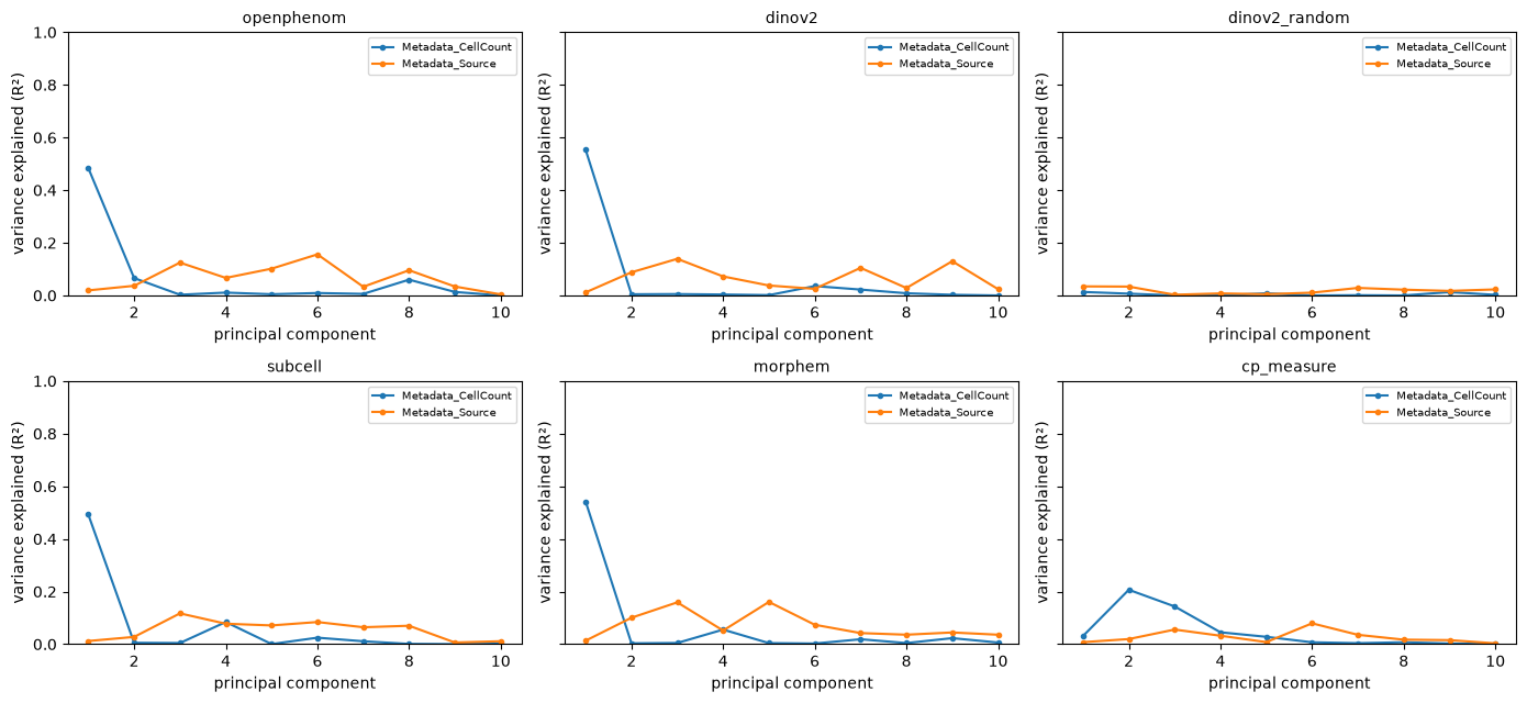
pc_regression, per component, on the cell count and on the laboratory.

fig, axes = plt.subplots(2, 3, figsize=(14, 6.5), sharey=True)
for ax, (model, wells) in zip(axes.ravel(), blocks.items(), strict=True):
    mt.pl.batch_variance(wells, keys=["Metadata_CellCount", "Metadata_Source"], use_rep="X_pca", n_comps=10, ax=ax)
    ax.set_title(model, fontsize=10)
fig.tight_layout()
plt.show()

variance = pd.concat(
    {
        model: mt.metrics.batch_variance_explained(
            wells, keys=["Metadata_CellCount", "Metadata_Source"], use_rep="X_pca"
        ).set_index("key")["value"]
        for model, wells in blocks.items()
    },
    axis=1,
).T.rename(columns={"Metadata_CellCount": "cell count", "Metadata_Source": "source"})
variance["first component, r with count"] = {
    model: float(np.corrcoef(wells.obsm["X_pca"][:, 0], wells.obs["Metadata_CellCount"])[0, 1])
    for model, wells in blocks.items()
}
variance.round(3)

key	cell count	source	first component, r with count
openphenom	0.323	0.035	-0.696
dinov2	0.376	0.030	0.744
dinov2_random	0.015	0.019	-0.116
subcell	0.216	0.034	0.702
morphem	0.301	0.044	0.736
cp_measure	0.060	0.021	-0.176

On every trained embedding the first component correlates with the cell count at about 0.70 to 0.74 in magnitude, against 0.18 for cp_measure and 0.12 for the untrained model, and over the fifty components the count accounts for between six and twelve and a half times as much of the variance as the laboratory does. The largest axis of these models tracks how full the well is. The untrained model does not do it, so the trained models learned it; cp_measure, a per-cell measurement summarised over the well, does it far less.

The untreated control wells differ 1.7-fold in cell count between sites, as the dataset page shows. If a good part of what separates the laboratories is how dense their wells are, a representation whose largest axis tracks density entangles the batch with the biology on that axis, which would be one reason the embeddings need the correction more than cp_measure does. This page does not test that.

How much of CellProfiler each embedding carries

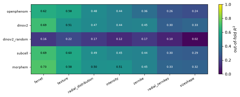
A learned embedding has no var to read a hit off: a compound that stands out is an ID, not “high texture in the mitochondrial channel”. So the question the comparison has skirted is what a black-box embedding actually holds of the named measurements it is being scored against. metrics.variance_carried answers it directly. It cross-fits a ridge from the embedding to each cp_measure feature and reports the out-of-fold R^2, averaged over each feature family: near one means the embedding linearly reconstructs that family, near zero means it does not carry it. The two blocks are the same 1,536 wells, so the metric aligns them on obs_names and needs nothing else. classical is the block to recover — normalized but not selected, so it still names every feature and its var["feature_group"].

carried = pd.DataFrame(
    {
        # blocks[model] holds the embedding in obsm["X_pca"]; classical.X holds the named cp_measure block.
        model: mt.metrics.variance_carried(
            blocks[model], classical, use_rep="X_pca", groupby="feature_group"
        ).set_index("feature_group")["variance_carried"]
        for model in blocks
        if model != "cp_measure"  # recovering cp_measure from itself is not the question
    }
).T
carried = carried[carried.mean().sort_values(ascending=False).index]  # feature families, best-carried first

fig, ax = plt.subplots(figsize=(9, 3.5))
im = ax.imshow(carried.to_numpy(), cmap="viridis", vmin=0, vmax=1, aspect="auto")
ax.set_xticks(np.arange(carried.shape[1]), carried.columns, rotation=30, ha="right", fontsize=8)
ax.set_yticks(np.arange(carried.shape[0]), carried.index, fontsize=8)
for row in range(carried.shape[0]):
    for col in range(carried.shape[1]):
        value = carried.iat[row, col]
        # white on the dark low end, black on the bright high end, so every cell stays readable
        ax.text(
            col, row, f"{value:.2f}", ha="center", va="center", fontsize=7, color="white" if value < 0.5 else "black"
        )
fig.colorbar(im, ax=ax, label="out-of-fold $R^2$")
fig.tight_layout()
plt.show()

carried.round(3)

feature_group	ferret	texture	radial_distribution	intensity	zernike	radial_zernikes	sizeshape
openphenom	0.619	0.583	0.480	0.440	0.362	0.265	0.239
dinov2	0.688	0.513	0.475	0.441	0.446	0.302	0.330
dinov2_random	0.163	0.221	0.169	0.121	0.166	0.101	0.017
subcell	0.692	0.597	0.489	0.454	0.442	0.302	0.292
morphem	0.725	0.579	0.504	0.509	0.447	0.326	0.318

The trained embeddings carry the ferret and texture families of cp_measure well — an image model reconstructs how large each object is and how patterned each channel is almost for free — and the zernike and shape families less, since those turn on the exact segmentation the embedding never performed. dinov2_random carries little of any family: the untrained control sits well below the trained models everywhere, which is the point. A learned embedding stops being a black box once you can say what of the classical block it linearly rebuilds; read each row against the control, not on its own.

Is the hit a hit, or did the cells die?

This is the question a screener asks first, and on an embedding it is sharper than usual. Call hits, then ask tl.cytotoxicity whether the compounds furthest from the controls are the ones that lost cells.

toxicity = []
for model, wells in blocks.items():
    scratch = wells.copy()
    mt.tl.hit_calling(scratch, use_rep="X_pca", n_permutations=200, seed=0)
    mt.tl.cytotoxicity(scratch, site_key=None)  # one field per well, so there is no field count to divide by
    table = scratch.uns["mantispy"]["cytotoxicity"]
    toxicity.append(
        {
            "model": model,
            "rho(distance, viability)": float(table[["distance", "viability"]].corr(method="spearman").iloc[0, 1]),
            "suspect": int(table["suspect"].sum()),
            "groups": len(table),
        }
    )
    if model == "openphenom":
        mt.pl.cytotoxicity(scratch)
pd.DataFrame(toxicity).set_index("model").round(3)

	rho(distance, viability)	suspect	groups
model
openphenom	-0.661	64	302
dinov2	-0.705	64	302
dinov2_random	-0.538	64	302
subcell	-0.736	64	302
morphem	-0.698	64	302
cp_measure	-0.700	64	302

The suspect count is identical on every block, the untrained one included, so here it follows viability alone. The rank correlation between distance and viability is negative on every block, from −0.54 for the untrained model to −0.74 for SubCell, and cp_measure sits at −0.70, inside the range of the trained embeddings. Cell loss moves a profile away from the controls whichever feature block measures it, because a compound that kills cells has changed the well. The top of this screen’s hit list is partly a cytotoxicity ranking whichever block you use.

Should the cell count be removed?

The reflex is to take the count out: drop the wells under a floor, or regress the count out of the profiles. Both are measured here on OpenPhenom, against keeping every well.

def remedy(treatment):
    """The recipe `prepared` ran, with a cell-count floor or with the count regressed out."""
    if treatment == "none":
        return blocks["openphenom"]  # already built above; rebuilding it is how the two quietly diverge
    wells = mt.ds.jump_lite("openphenom")
    if treatment == "floor":
        wells = wells[wells.obs["Metadata_CellCount"].to_numpy(dtype=float) >= 50].copy()
    mt.pp.normalize(wells, method="mad_robustize", by="Metadata_Plate", reference="negcon")
    # The same step `prepared` runs. It drops nothing from this embedding, and leaving it out is how the
    # floor and regress arms would end up compared against a "none" arm built a different way.
    mt.pp.feature_select(wells, operations=("drop_degenerate", "drop_na_columns"), na_cutoff=0.0)
    wells = mt.pp.subset_features(wells)
    if treatment == "regress":
        mt.pp.regress_out(wells, keys=("Metadata_CellCount",), by="Metadata_Plate")
    return align(wells)


remedies = []
for treatment in ("none", "floor", "regress"):
    trial = remedy(treatment)
    left = float(mt.metrics.pc_regression(trial, key="Metadata_CellCount", use_rep="X_pca")["value"].iloc[0])
    for rep in ("X_pca", "X_tvn", "X_harmony"):
        result = scored(treatment, trial, rep)
        remedies.append(
            {
                "treatment": treatment,
                "alignment": rep,
                "wells": trial.n_obs,
                "cell count variance": left,
                "mAP": result["mAP"],
                "significant": result["significant"],
                "target recall": result["target recall"],
                "recall null": result["recall null"],
                "recall p": result["recall p"],
            }
        )
pd.DataFrame(remedies).set_index(["treatment", "alignment"]).round(3)

		wells	cell count variance	mAP	significant	target recall	recall null	recall p
treatment	alignment
none	X_pca	1536	0.323	0.016	0	0.057	0.066	0.851
	X_tvn	1536	0.323	0.018	3	0.127	0.091	0.010
	X_harmony	1536	0.323	0.037	4	0.069	0.081	0.941
floor	X_pca	1397	0.250	0.016	0	0.048	0.073	1.000
	X_tvn	1397	0.250	0.020	3	0.152	0.111	0.010
	X_harmony	1397	0.250	0.034	17	0.048	0.061	0.990
regress	X_pca	1536	0.064	0.010	1	0.127	0.093	0.010
	X_tvn	1536	0.064	0.018	3	0.161	0.114	0.010
	X_harmony	1536	0.064	0.022	0	0.109	0.084	0.010

Each remedy buys something the other does not. Regressing the count out takes its share of the variance from 0.32 to 0.06 and lifts annotation recall above its own null under every alignment, where keeping every well clears it only under TVN. It costs retrieval: under Harmony the compounds called drop from four to none. The floor discards 139 wells, raises the calls under Harmony from four to seventeen at a small cost in mAP, and leaves recall below its null there. Under TVN neither costs anything this table scores.

In a compound screen the count is partly a treatment effect, since the compound reduced it, so regressing it out removes part of the phenotype and not only a nuisance. The JUMP recipe regresses the cell count out of the ORF and CRISPR arms and not out of compounds [Chandrasekaran et al., 2023]. This page keeps every well and does not regress; report the count beside the readouts instead.

Summary

• On telling a compound from DMSO the blocks were close; on telling compounds apart across laboratories without a correction the embeddings called at most five compounds to cp_measure’s 32. Harmony narrowed that for every trained embedding but OpenPhenom.

• Read Harmony as a range over seeds, and read cp_measure’s row as one recipe: the rank transform halves its calls under Harmony.

• Measure chance with known_relationships(n_permutations=...), and keep an untrained model in the comparison. Against a fixed 10% it would have looked like the best model without TVN.

• The trained embeddings’ largest axis tracks confluence, and distance from the controls tracks cell loss on every block.

• The three alignments disagree and none dominates: Harmony lets the embeddings’ compounds reproduce across sites, TVN lets their annotation recall clear its null.

All of it is for off-the-shelf embeddings on lossy JUMP images and one CellProfiler recipe.